GCP Performance Optimization with BigQuery, Cloud Functions, and Kubernetes

TL;DR

• BigQuery: partition, cluster, select only what you need. Partitioned tables (PARTITION BY DATE) drastically reduce scanned data. Clustering sorts data within partitions for efficient filtering. Never SELECT *  BigQuery charges by data scanned. Use materialized views for frequent aggregations; slot reservations for predictable capacity.
• Cloud Functions: minimize cold starts, optimize memory. Set minInstances to keep functions warm for latency-sensitive workloads. Higher memory = faster CPU some functions run faster (and cheaper) with more memory. Initialize clients globally, outside the handler. Use concurrency settings (up to 1000 per instance) to reduce instance count. Cloud Functions 2nd gen supports longer timeouts (60 min) and traffic splitting.
• GKE: Autopilot simplifies, but resource requests matter. Autopilot manages nodes automatically great for most workloads. Always set pod resource requests and limits this enables proper scheduling and Horizontal Pod Autoscaling. Use Vertical Pod Autoscaler to recommend optimal settings; Horizontal Pod Autoscaler to scale replicas based on CPU/metrics. Spot VMs cut costs 60-91% for fault-tolerant workloads.
• Cloud SQL & Spanner: size appropriately, pool connections. Choose instance memory based on working set size. Use read replicas to scale read capacity; route queries accordingly. Enable Query Insights to find slow queries without external tools. For Spanner, design schemas for even data distribution; use interleaved tables to co-locate parent-child rows.
• Cache everywhere possible: Memorystore (Redis/Memcached) reduces database load. Cloud CDN caches content at edge locations globally. Configure Cache-Control headers appropriately. Use signed URLs to cache authenticated content securely.
• Monitor with Cloud Operations: Enable Cloud Trace for distributed tracing; Cloud Profiler for production CPU/memory analysis. Set SLO-based alerting. Track custom metrics via the Monitoring API.

Google Cloud Platform offers powerful services built on the same infrastructure that runs Google's own products. Optimizing performance on GCP requires understanding how BigQuery processes queries, how Cloud Functions scale, and how Google Kubernetes Engine manages workloads. Each service has distinct performance characteristics and optimization strategies.

BigQuery Performance Optimization

BigQuery separates storage from compute, enabling massive scalability. Performance optimization focuses on query efficiency and data organization rather than infrastructure tuning.

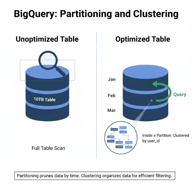
Partitioned tables dramatically improve query performance. Time-based partitioning limits data scanned for time-range queries. Integer-range partitioning suits non-temporal data.

-- Create partitioned table
CREATE TABLE mydataset.events
PARTITION BY DATE(event_timestamp)
CLUSTER BY user_id
AS SELECT * FROM mydataset.raw_events;

Clustering organizes data within partitions. Clustered columns sort data blocks, enabling efficient filtering. Combine partitioning and clustering for optimal performance.

Column selection matters critically. BigQuery charges for data scanned. Select only needed columns rather than using SELECT *. Query costs and performance improve together.

-- Expensive: scans all columns
SELECT * FROM mydataset.events WHERE date = '2025-01-15';

-- Efficient: scans only needed columns
SELECT user_id, event_type, event_timestamp
FROM mydataset.events
WHERE date = '2025-01-15';

Materialized views pre-compute aggregations. For frequently-run aggregate queries, materialized views return results instantly while BigQuery maintains freshness automatically.

BI Engine provides in-memory analysis for dashboards. Sub-second query responses enable interactive exploration of large datasets.

Slot reservations provide predictable capacity. On-demand pricing works for variable workloads. Reserved slots ensure capacity for consistent, heavy workloads.

Avoid transformation in SELECT clauses when possible. Functions applied to columns prevent partition pruning. Push transformations to the WHERE clause when filtering.

Cloud Functions Efficiency

Cloud Functions execute code in response to events. Performance optimization reduces cold starts, execution time, and memory consumption.

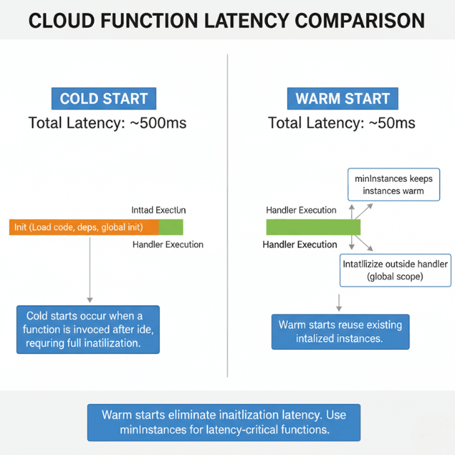
Minimum instances eliminate cold starts for latency-sensitive functions. Pre-warmed instances respond immediately. Balance always-on costs against cold start impact.

# Cloud Functions configuration
runtime: nodejs18
minInstances: 2
maxInstances: 100
availableMemory: 256MB

Memory allocation affects CPU allocation proportionally. Higher memory provides faster CPUs. Some functions run faster with more memory despite not needing the RAM.

Global scope initialization runs once per instance. Move database connections, SDK initialization, and configuration loading outside the function handler.

// Initialize outside handler - runs once per instance
const { Firestore } = require('@google-cloud/firestore');
const db = new Firestore();

// Handler runs per invocation
exports.handleRequest = async (req, res) => {
  const doc = await db.collection('users').doc(req.body.userId).get();
  res.json(doc.data());
};

Concurrency settings control how many requests share an instance. Higher concurrency (up to 1000) reduces instance count and cold starts. Ensure code handles concurrent requests safely.

Dependency optimization reduces deployment size. Smaller packages load faster. Remove unused dependencies. Consider lighter alternatives to heavy libraries.

Cloud Functions 2nd generation, built on Cloud Run, provides longer timeouts (up to 60 minutes), larger instances, and traffic splitting for gradual rollouts.

VPC connectors add latency for private network access. Use Serverless VPC Access only when required. Consider Cloud Run for VPC-heavy workloads.

Google Kubernetes Engine Optimization

Google Kubernetes Engine manages Kubernetes clusters with Google's infrastructure expertise. Optimization spans cluster configuration, pod resources, and application architecture.

Autopilot mode manages nodes automatically. GKE provisions and scales nodes based on pod requirements. Standard mode provides more control for specialized workloads.

Node pool configuration matches workload needs. General-purpose e2 machines suit most workloads. Compute-optimized c2 machines accelerate CPU-intensive work. Memory-optimized m2 machines support large databases.

# Pod resource requests and limits
resources:
  requests:
    memory: "256Mi"
    cpu: "100m"
  limits:
    memory: "512Mi"
    cpu: "500m"

Vertical Pod Autoscaler recommends resource settings. It analyzes actual usage and suggests appropriate requests and limits. This prevents over-provisioning while avoiding OOM kills.

Horizontal Pod Autoscaler scales replicas based on metrics. CPU and memory thresholds trigger scaling. Custom metrics from Cloud Monitoring enable application-specific scaling.

apiVersion: autoscaling/v2
kind: HorizontalPodAutoscaler
spec:
  minReplicas: 2
  maxReplicas: 20
  metrics:
  - type: Resource
    resource:
      name: cpu
      target:
        type: Utilization
        averageUtilization: 70

Node auto-provisioning creates optimal node pools. GKE adds node pools matching pending pod requirements rather than fitting pods into existing nodes.

Spot VMs reduce costs by 60-91% for fault-tolerant workloads. Combine with Pod Disruption Budgets to maintain availability during preemptions.

Container-native load balancing routes traffic directly to pods. This eliminates the extra hop through kube-proxy, reducing latency.

Cloud SQL and Spanner Performance

Cloud SQL provides managed MySQL, PostgreSQL, and SQL Server. Spanner provides horizontally scalable relational database capabilities.

Cloud SQL instance sizing affects performance directly. Choose CPU and memory based on workload characteristics. High-memory configurations suit OLTP workloads with large working sets.

Read replicas scale read capacity. Route read queries to replicas using connection pooling logic. Replicas lag slightly behind primary, so route accordingly.

# Route reads to replica, writes to primary
def get_connection(is_read=True):
    if is_read:
        return replica_pool.getconn()
    return primary_pool.getconn()

Query Insights identifies slow queries without external tools. The Cloud Console displays query performance data including lock waits and execution statistics.

Connection pooling prevents connection exhaustion. Cloud SQL limits connections based on instance size. Use connection poolers like PgBouncer or Cloud SQL Proxy with connection limits.

Spanner scales horizontally by adding nodes. Performance increases linearly with node count. Design schemas to distribute data evenly across splits.

Spanner interleaved tables co-locate parent and child rows. This eliminates join overhead for parent-child queries by storing related rows together.

Cloud CDN and Load Balancing

Cloud CDN caches content at Google's edge locations. Combined with global load balancing, this architecture provides low-latency access worldwide.

Cache policies control what gets cached and for how long. Configure Cache-Control headers appropriately. Cloud CDN respects origin cache directives.

# Origin server cache headers
Cache-Control: public, max-age=3600

Signed URLs and signed cookies protect cached content. Enable caching for authenticated content without exposing data to unauthorized users.

Backend service configuration affects load balancing behavior. Connection draining gracefully handles instance removal. Health checks detect unhealthy backends.

Cloud Armor provides DDoS protection and WAF capabilities. Rules filter malicious traffic at the edge before reaching backends.

Global load balancing uses anycast IPs. Users connect to the nearest Google edge location, then traffic routes internally to the optimal backend.

Premium Tier networking uses Google's private network globally. Standard Tier uses public internet routing. Premium Tier provides lower latency for cross-region traffic.

Memorystore for Caching

Memorystore provides managed Redis and Memcached. Caching reduces backend load and improves response times.

Instance tiers range from Basic (no replication) to Standard (high availability). Choose based on availability requirements. Standard tier provides automatic failover.

Memory sizing determines capacity. Monitor cache hit rates and eviction rates. Resize instances when eviction increases or hit rates drop.

import redis

# Connection with retry logic
r = redis.Redis(
    host='10.0.0.3',
    port=6379,
    socket_timeout=5,
    socket_connect_timeout=5,
    retry_on_timeout=True
)

# Cache-aside pattern
def get_user(user_id):
    cached = r.get(f"user:{user_id}")
    if cached:
        return json.loads(cached)

    user = db.query_user(user_id)
    r.setex(f"user:{user_id}", 3600, json.dumps(user))
    return user

VPC peering connects Memorystore to GKE and other services. Private connectivity keeps traffic off the public internet.

Redis persistence options include RDB snapshots and AOF logs. Persistence adds overhead but enables recovery after restarts.

Memcached suits simple caching without persistence requirements. Higher memory efficiency and simpler operation for ephemeral caching.

Monitoring with Cloud Operations

Cloud Operations (formerly Stackdriver) provides monitoring, logging, and tracing across GCP services.

Cloud Monitoring collects metrics automatically. Custom metrics track application-specific measurements. Dashboards visualize performance across services.

from google.cloud import monitoring_v3

client = monitoring_v3.MetricServiceClient()
series = monitoring_v3.TimeSeries()
series.metric.type = "custom.googleapis.com/order_processing_time"
series.points.append(point)
client.create_time_series(name=project_path, time_series=[series])

Cloud Trace provides distributed tracing. Traces show request flow across services, identifying latency bottlenecks.

Cloud Profiler continuously samples production code. Flame graphs reveal CPU and memory consumption by function.

Alerting policies notify teams of issues. Multi-condition alerts reduce false positives. Notification channels include email, SMS, PagerDuty, and webhooks.

SLO monitoring tracks service level objectives. Define SLIs based on latency, availability, or error rates. Error budgets show remaining room for risk-taking.

Conclusion

GCP's performance optimization landscape is rich with managed services that abstract infrastructure while exposing critical knobs for tuning. BigQuery's separation of storage and compute makes it uniquely powerful but only if you respect its query patterns: partition, cluster, and select narrowly.

Cloud Functions and GKE offer different tradeoffs in the serverless-to-container spectrum; the key is matching the service to workload characteristics. Functions excel at event-driven, low-latency logic; GKE gives you full control for complex, stateful applications.

Across all services, the common thread is measurement: Cloud Operations provides the visibility you need to identify bottlenecks, set SLOs, and validate optimizations. Start with the highest-impact levers:

BigQuery partitioning, GKE resource requests, and Cloud Functions concurrency. Then iterate. The investment in GCP optimization compounds every query faster, every function warmer, every cluster more efficiently packed directly reduces costs and improves user experience.

FAQs

What's the single biggest mistake people make with BigQuery performance?

Using SELECT * on large tables. BigQuery charges by the amount of data scanned per query. SELECT * scans every column, even those you don't need. If a table has 50 columns but you only need 3, you're paying for 47 columns of unnecessary scanning. Always specify only the columns you need. Combined with partitioning and clustering, this is the highest-leverage optimization.

When should I use Cloud Functions vs. GKE?

Use Cloud Functions for:

• Event-driven, stateless logic (file upload triggers, pub/sub messages, HTTP APIs with variable traffic)
• Short execution times (<10 minutes for 1st gen, <60 minutes for 2nd gen)
• Teams that want zero infrastructure management

Use GKE for:

• Stateful applications requiring persistent storage
• Long-running or scheduled batch processing
• Microservices with complex networking requirements
• When you need control over node configuration, GPU/TPU access, or specialized hardware

Many teams use both: GKE for core services, Cloud Functions for event handlers and glue logic.

How do I choose between Cloud SQL, Spanner, and Firestore?

• Cloud SQL: Managed MySQL/PostgreSQL. Best for traditional relational apps, moderate scale (<10TB), strong consistency requirements. Easy migration path from self-hosted databases.
• Spanner: Horizontally scalable relational database. Choose for global scale (>10TB, >1M writes/sec) with strong consistency across regions. More complex schema design and higher cost than Cloud SQL.
• Firestore: NoSQL document database. Choose for mobile/web apps, real-time updates, simple queries, and when you don't need complex joins. Scales automatically with no capacity planning. Each has different performance characteristics and cost models match to your workload, not just familiarity.